Fig. 1. Organic chiral ligand pn = 1,2-diaminopropane. Crystallographic chirality is introduced using the chiral ligand.
It is standard knowledge in high school physics that in a direct current motor the rotor is driven by the force exerted on the current flowing in a magnetic field. At the same time a wire moving in a magnetic field acquires an electromotive force that opposes the original voltage from the external source. This effect, known as the counter emf, is conceptually well established, but has not been demonstrated experimentally at a high school level where steady-state measurements are the standard practice. We have performed time-resolved measurement of the current through a DC motor in which the magnetic field is provided by commercial ferrite magnets, and analyzed the result to derive the magnetic flux density (Figs. 2 and 3 and Photo1). The magnetic flux density (0.0580 ± 0.0015) T thus determined, agrees satisfactorily well with 0.068 T obtained independently using a Hall effect device. The small difference may be attributed to the spatial distribution of the flux density.
Fig. 1. Organic chiral ligand pn = 1,2-diaminopropane. Crystallographic chirality is introduced using the chiral ligand.
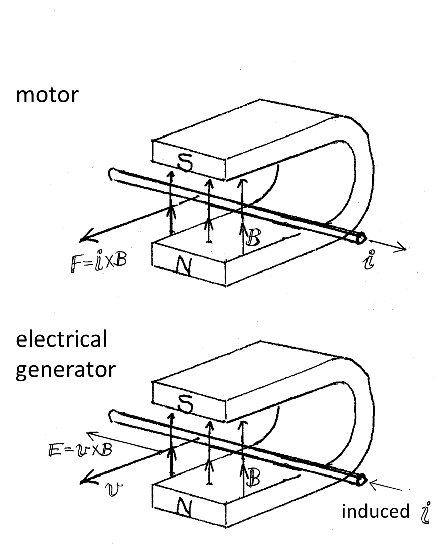
Fig. 1 The principles of a DC motor and electric generator.
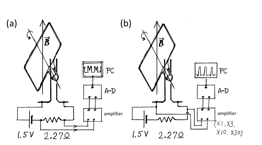
Fig. 2 Schematics of the current (a) and voltage (b) measurement.
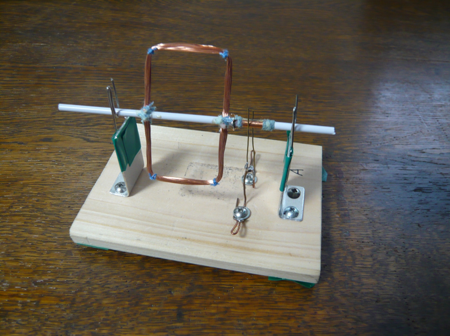
Photo. 1 The rotor of the DC motor. Ferrite magnets, normally placed below and above the rotor coil, have been removed.
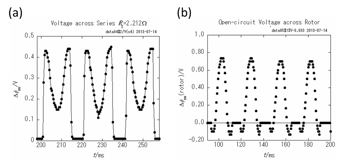
Fig. 3 Results of the time-resolved measurements. (a) Voltage across the fixed series resistor. The motor is driven by the current from the cell. The current decreases when the rotor coil cuts the magnetic flux vertically (i.e., at 208, 228 and 229 ms), generating a counter emf. (b) Voltage across the inertially spinning rotor coil. The battery has been turned off and the circuit is open with no current flowing. Notice the slightly decreasing peak heights as the time elapsed from 100ms to 180ms, indicating the deceleration due to mechanical friction and air viscosity.
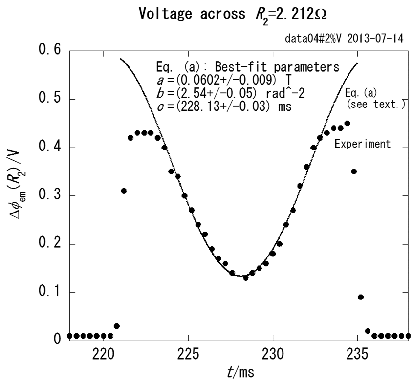
Fig. 4 The best-fit curve and parameters of the counter emf equation (eq. (a)) derived from a portion of Fig. 3(a). Dots are the experimental data. The data plotted in Fig. 3(b) have been similarly analyzed using eq. (b).